

Market Data

August 4, 2017
Strong Job Creation in June-July
Written by Peter Wright
The Bureau of Labor Statistics (BLS) employment report for July was released on Friday with a gain in jobs that exceeded analysts’ expectations. The May result was revised down by 7,000 and June was revised up by 9,000 positions. Using a three-month moving average (3MMA), the July result was 195,000 jobs, which was pulled down by poor growth in May of just 145,000 positions.
Economy.com summarized as follows: “July was another good month for the U.S. labor market. Nonfarm employment rose by 209,000 between June and July, better than our above-consensus forecast for a 185,000 increase. Private employment rose 205,000 and gains were broad-based. The workweek was unchanged, while average hourly earnings for all private workers rose 0.3 percent following a 0.2 percent increase in June. At first glance, there were not a ton of surprises in the household survey, as the unemployment rate slipped from 4.4 percent to 4.3 percent. The implications for monetary policy are straightforward—the labor market supports the Fed’s balance sheet plan and keeps another rate hike alive this year, most likely in December.”
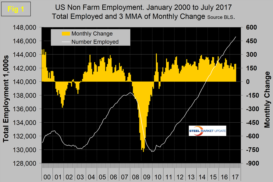
Figure 1 shows the 3MMA of the number of jobs created monthly since 2000 as the brown bars and the total number employed as the white line.
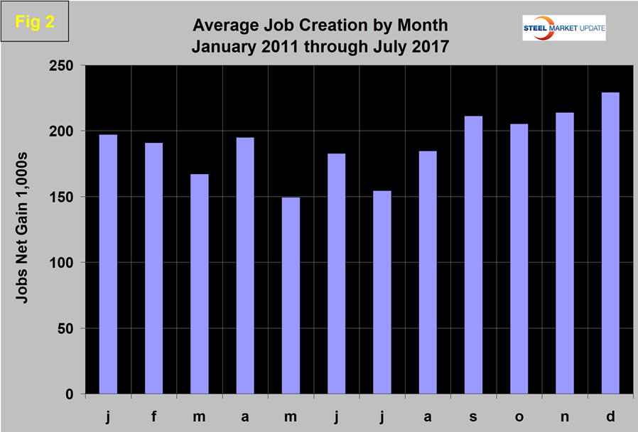
These numbers are seasonally adjusted by the BLS, which has been criticized in the past for the ineffectiveness of its seasonal adjustment calculations. To examine if any seasonality is left in the data after adjustment, we have developed Figure 2. In the seven years since and including 2011, job creation in July has been down by 15 percent. This year, July was down by 10 percent, therefore seasonally better than normal. July is adversely affected by the closure of auto assembly plants for re-tooling and maintenance. Figure 2 supports the view that the adjustments performed by the BLS still need some work. We can expect strong job gains in both August and September.
Total nonfarm payrolls are now 8,250,000 more than they were at the pre-recession high of January 2008. November 2014 was the first month for total nonfarm employment to exceed 140 million and in July was 146.6 million. The BLS reported that the average workweek for all employees on private nonfarm payrolls was unchanged at 34.5 hours in July. In manufacturing, the workweek was also unchanged at 40.9 hours, and overtime remained at 3.3 hours. The average workweek for production and nonsupervisory employees on private nonfarm payrolls was 33.7 hours for the fourth consecutive month. In July, average hourly earnings for all employees on private nonfarm payrolls rose by 9 cents to $26.36. Over the year, average hourly earnings have risen by 65 cents, or 2.5 percent. In July, average hourly earnings of private-sector production and nonsupervisory employees increased by 6 cents to $22.10.
Table 1 breaks total employment down into service and goods-producing industries and then into private and government employees.
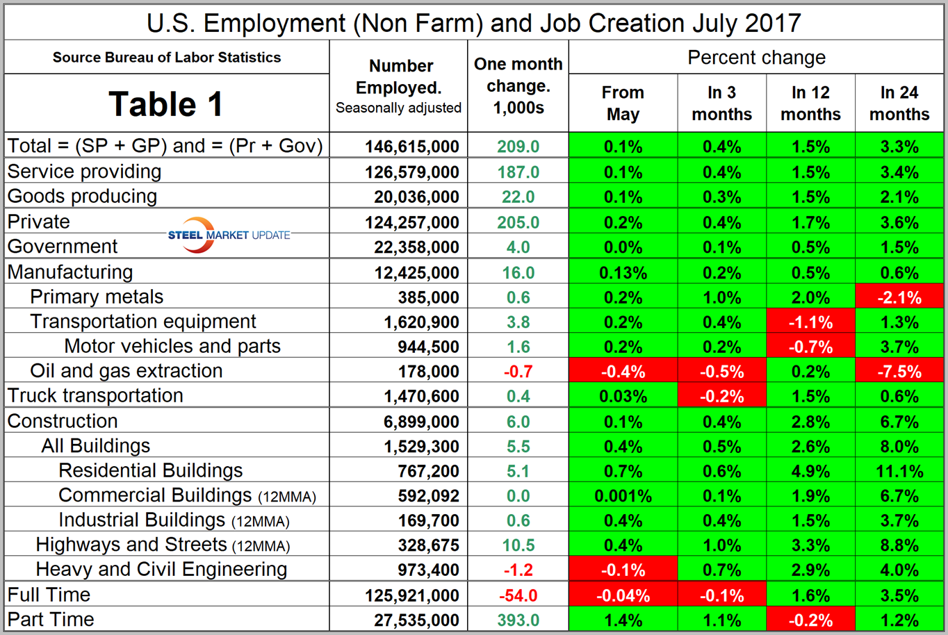
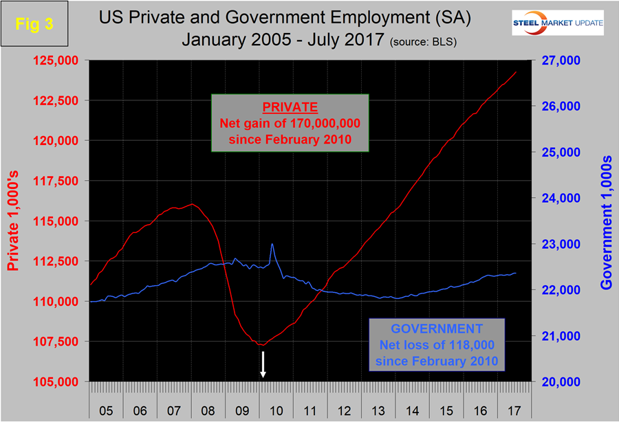
Most of the goods-producing employees work in manufacturing and construction. The components of these two sectors that we consider to be most relevant to steel executives are broken out in Table 1. In July, 205,000 jobs were created in the private sector and government gained 4,000 jobs. The number employed by the federal government was unchanged at 2.8 million; state governments lost 3,000 for a total of 5.96 million; and local governments gained 7,000 to reach a total of 14.45 million. Since February 2010, the employment low point, private employers have added 17,000,000 jobs as government has shed 118,000 (Figure 3).
In July, service industries expanded by 187,000 as goods-producing industries driven mainly by construction and manufacturing expanded by 22,000. Since February 2010, service industries have added 14,473,000 and goods-producing 2,409,000 positions. This is part of the reason why wage growth has been slow since the recession, as service industries on average pay less than goods producers such as manufacturers.
In July, manufacturing gained 16,000 positions and has not had a losing month since October last year. In the first seven months of 2017, manufacturing has gained 82,000 jobs and is 0.5 percent higher than the same month in 2016. Table 1 shows that primary metals gained 600 jobs in July and is up by 9,000 year-to-date. Transportation equipment including aircraft gained 3,800 jobs in July of which 2,000 were in the motor vehicles and parts industries. Trucking was very strong in both February and March, but lost ground in April, May and June with a small gain in July. Oil and gas extraction has been stalled since August last year with zero net gain in that time frame. Note that the subcomponents of both manufacturing and construction shown in Table 1 don’t add up to the total because we have only included those that we think have most relevance to the steel industry.
Construction was reported to have gained 6,000 jobs in July and is up by 191,000 or 2.8 percent in the last 12 months. Some of the major construction sub categories are routinely reported one month in arrears, which distorts the data in Table 1. These include, industrial buildings, commercial buildings, and highways and streets. Construction has added 1,399,000 jobs and manufacturing 972,000 since the recessionary employment low point in February 2010 (Figure 4).
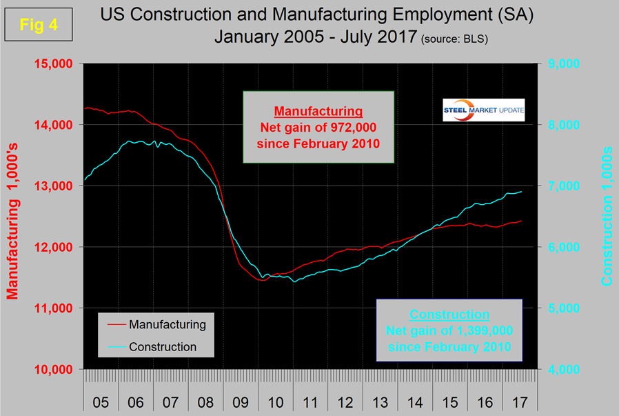
Construction has leapt ahead of manufacturing as a job creator, but the growth of construction productivity is very low (or non-existent), in contrast to manufacturing where it has been historically high. The difference is the difficulty of automating construction jobs.
According to Ken Simonson, chief economist of the Associated General Contractors of America, “Forty-one states added construction jobs between June 2016 and June 2017 amid continuing widespread demand for construction services. Contractors in most of the country say they have plenty of projects booked and would like to hire more workers if they could find them, so it is likely that some states with monthly employment declines have a shortage of workers available to hire rather than a slowdown in work. Given the low unemployment rate in most states, other industries are competing hard for workers, making it difficult for contractors to find new construction workers, let alone experienced ones.”
The official unemployment rate, U3, reported in the Household survey of the BLS (see explanation below) came in at 4.3 percent, which was down from 4.9 percent in July last year. This number doesn’t account for those who have stopped looking. The more comprehensive U6 unemployment rate declined from 9.7 percent in July last year to 8.6 percent in this latest report (Figure 5).
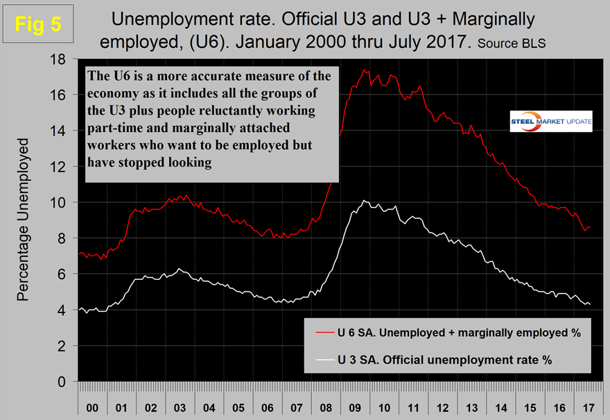
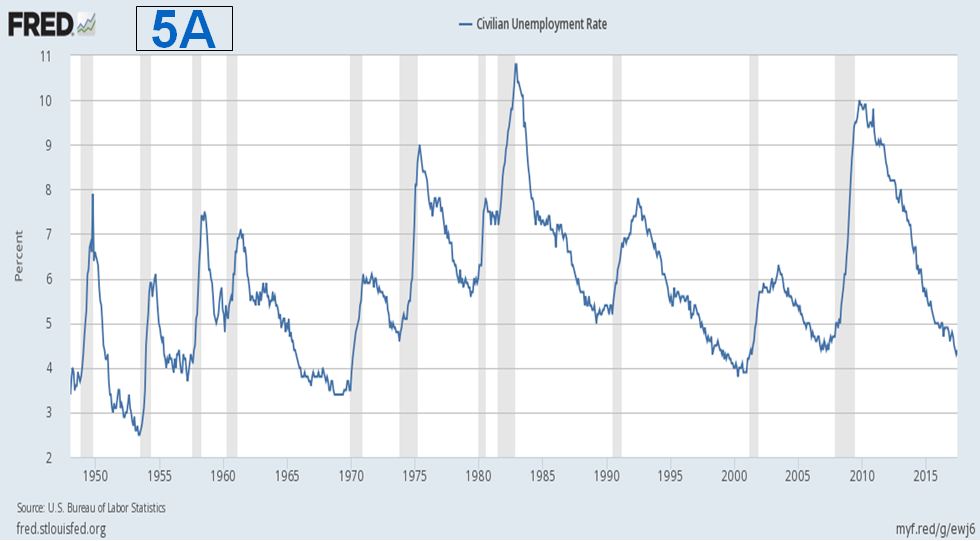
U6 includes workers working part time who desire full-time work and people who want to work but are so discouraged they have stopped looking. The differential between these rates was usually less than 4 percent before the recession and is now down to 4.3 percent. On Aug. 1, equities analyst Daniel Carter wrote: “Even though the Unemployment Rate is terrible at its designed purpose, it presents one of the clearest pictures of the business cycle. It falls slowly and consistently when the economy is expanding, and it rises sharply when the economy shrinks. Right before a recession, the Unemployment Rate finds a bottom and the trend slowly begins to reverse. When a recession occurs, the uptrend that was established months before turns into a rapid increase. The Unemployment Rate bottoms an average of eight months before a recession. The maximum number of months between an Unemployment Rate bottom and a recession was 18 months, and the minimum number of months between an Unemployment Rate bottom and a recession was 2 months.” We have included Figure 5A, which was extracted from Carter’s publication. This is the best correlation we have ever seen as a predictor of recessions.
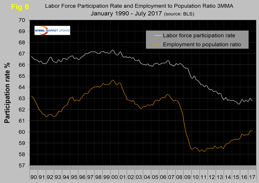
The employment participation rate at 62.9 percent in July was up slightly from 62.8 percent in July last year. We’re not sure what this is a percentage “of” because of the multiple descriptions of the labor pool. Another measure is the number employed as a percentage of the population, which we think is much more definitive. In July, this measure was 60.2 percent, up from 59.8 percent in July last year and from 59.3 percent in July 2015. The employment-to-population ratio stalled for most of last year, but has made progress in 2017. Figure 6 shows both measures on one graph.
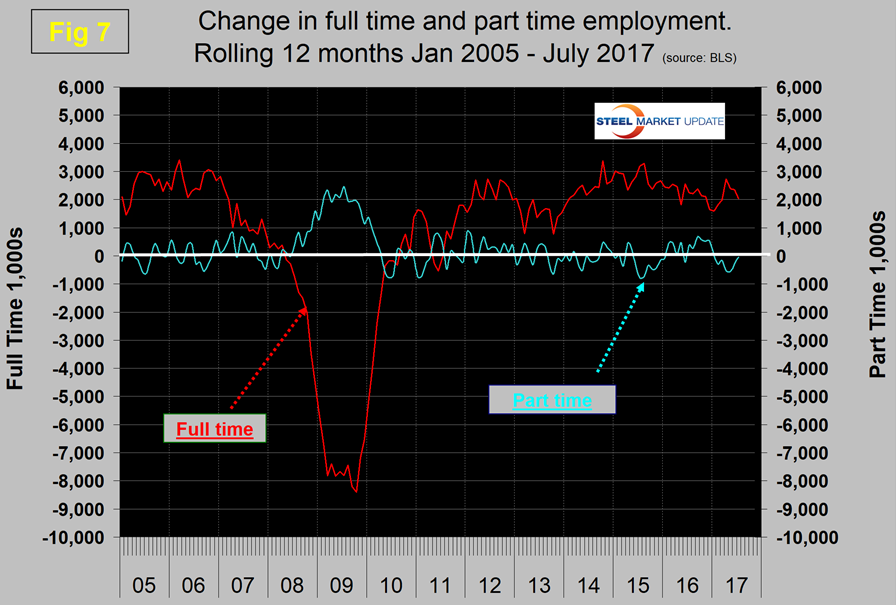
In the 31 months since and including January 2015, there has been an increase of 5,259,000 full-time and a gain of 51,000 part-time jobs. Figure 7 shows the rolling 12-month total change in both part-time and full-time employment. This data comes from the household survey and part-time is defined as less than 35 hours per week. Because the full-time/part-time data comes from the household survey and the headline job creation number comes from the establishment survey, the two cannot be compared in any particular month. To overcome the volatility in the part-time numbers, we have to look at longer time periods than a month or even a quarter, which is why we look at a rolling 12 months for this component of the employment picture shown in Figure 7.
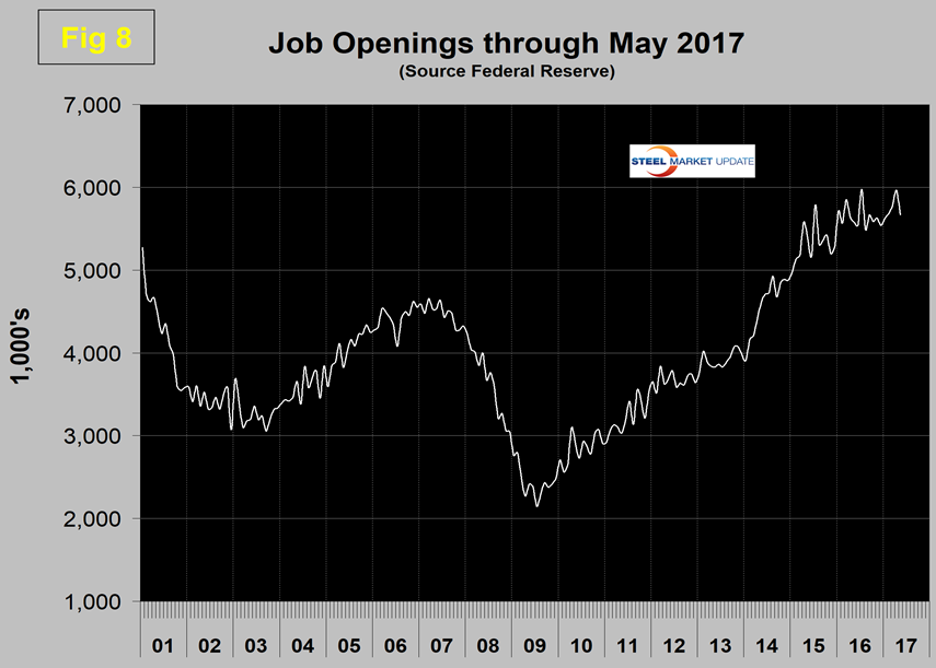
The job openings report known as JOLTS is reported on about the 10th of the month by the Federal Reserve and is over a month in arrears. Figure 8 shows the history of unfilled job openings through May when openings stood at 5,666,000, not far off the all-time high of 5,852,000 in March last year. There has been an improving trend since mid-2009.
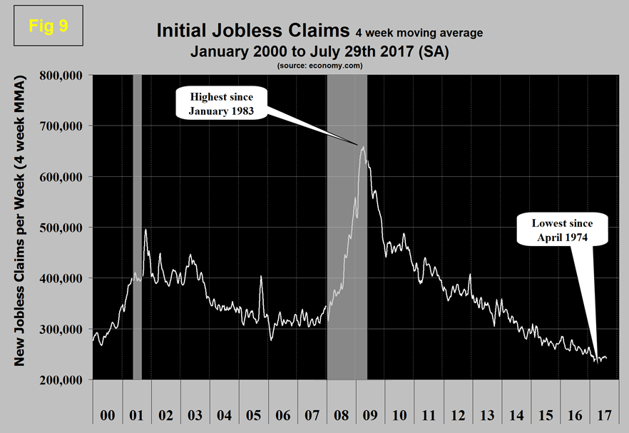
Initial claims for unemployment insurance, reported weekly by the Department of Labor, have flattened this year at the lowest level since 1974. In the week ending July 29, initial claims were 240,000 with a four-week moving average of 241,750 claims. This marks the longest streak since 1973 of initial claims below 300,000 (Figure 9). The result for the week ending Feb. 4, 2017, at 231,000 was the lowest since March 1973.
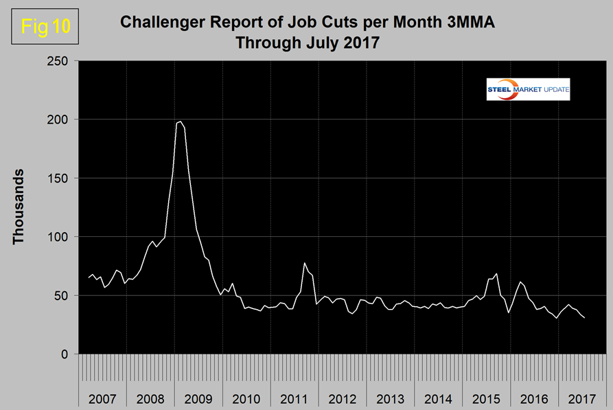
The last piece of the employment puzzle that we examine is the Challenger report, which measures job cuts monthly (Figure 10). This data also tends to be quite erratic, therefore again we examine a rolling average and can see that job cuts decreased for most of 2016 and continued their downward trend in 2017.
SMU Comment: Overall, we think the employment situation is very good and has been described as “full” by some analysts. July was the 82nd consecutive month of job growth, but Figure 1 shows a slowing trend since mid-2014. If as reported there is a shortage of qualified employees, we can expect an increase in wage-driven inflation soon. The results for manufacturing and construction are sign posts for steel sales activity. In the big picture, layoffs are historically low and job openings are close to all-time highs, therefore 2017 is tracking well.
Explanation: On the first Friday of each month, the Bureau of Labor Statistics releases the employment data for the previous month. Data is available at www.bls.gov. The BLS reports on the results of two surveys. The Establishment survey reports the actual number employed by industry. The Household survey reports on the unemployment rate, participation rate, earnings, average workweek, the breakout into full-time and part-time workers and lots more details describing the age breakdown of the unemployed, reasons for and duration of unemployment. At SMU, we track the job creation numbers by many different categories. The BLS database is a reality check for other economic data streams such as manufacturing and construction, and we include the net job creation figures for those two sectors in our “Key Indicators” report. It is easy to drill down into the BLS database to obtain employment data for many subsectors of the economy. For example, among hundreds of sub-indexes are truck transportation, auto production and primary metals production. The important point about each of these hundreds of data streams is in which direction they are headed. Whenever possible, we try to track three separate data sources for a given steel-related sector of the economy. We believe this gives a reasonable picture of market direction. The BLS data is one of the most important sources of fine-grained economic data that we use in our analyses. The states also collect their own employment numbers independently of the BLS. The compiled state data compares well with the federal data. Every three months, SMU examines the state data and provides a regional report, which indicates strength or weakness on a geographic basis. Reports by individual state can be produced on request.