Gross Domestic Product Q3 2015 Third Estimate

The annualized growth rate in the 3rd estimate of the 3rd quarter was 1.99 percent, down from 3.91 percent, in the 3rd estimate of Q2. GDP is measured and reported in chained 2009 dollars and in the third estimate of Q3 was $16.414 trillion. The growth calculation is misleading because it takes the Q over Q change and multiplies by 4 to get an annualized rate. This makes the high quarters higher and the low quarters lower. Figure 1 clearly shows this effect.

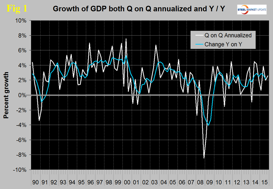
The blue line is the trailing 12 months growth and the white line is the headline quarterly result. On a trailing 12 month basis year over year, GDP was 2.15 percent higher in the 3rd quarter than it was in Q3 2014. In the last five years, since Q1 2011 the trailing 12 month growth of GDP has ranged from a high of 2.88 percent to a low of 1.07 percent therefore the latest result is central within this variability.

Figure 2 shows the headline quarterly results since 1990 and the latest IMF forecast through 2020.

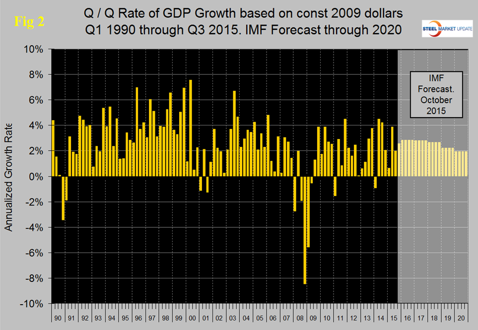
In their October revision, the IMF downgraded their forecast of US growth in 2015 from their April estimate of 3.14 percent to 2.57 percent and downgraded 2016 from 3.06 percent to 2.84 percent.

Historically it has been necessary to have about a 2.5 percent growth in GDP to get any growth in steel demand so this forecast suggests a status quo through next year for our businesses.

There are six major subcomponents of the GDP calculation and the magnitude of these is shown in Figure 3.

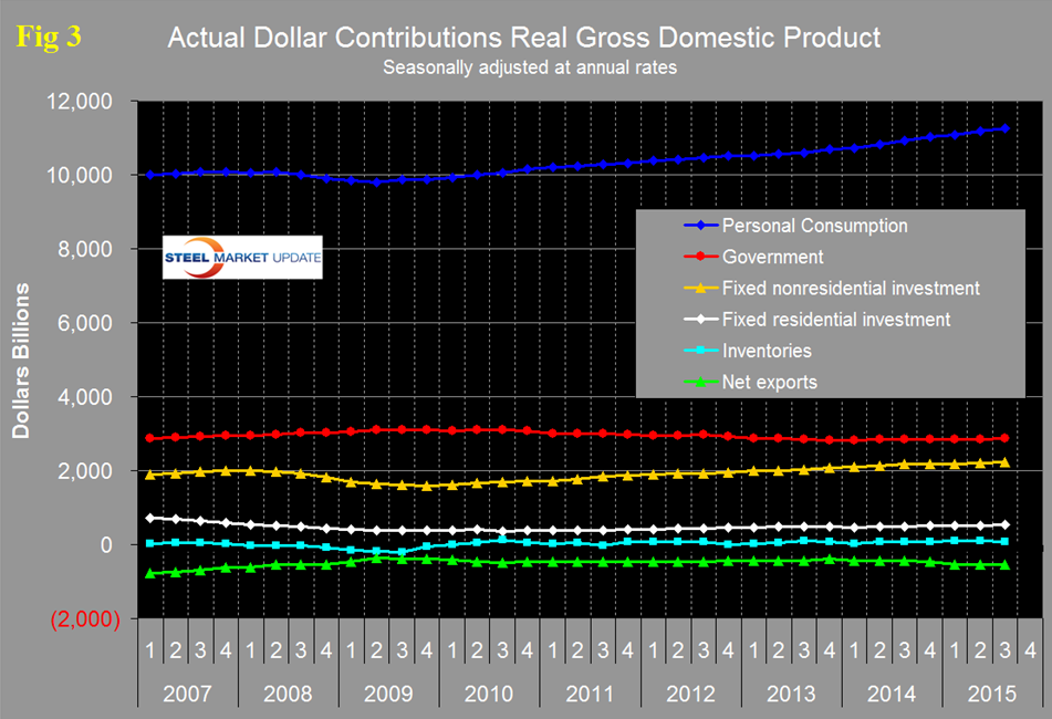
Personal consumption is dominant and in Q3 accounted for 68.61 percent of the total. Figure 4 shows the change in the major subcomponents of GDP in Q3 2015.

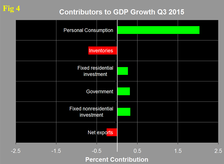
This shows how dominant the contribution of personal consumption was in the 3rd quarter and also that the change in private inventories was a major detractor. Declining inventories have a negative effect on the overall GDP calculation. Figure 5 shows the same data as Figure 4 extended back through Q1 2007 and describes the quarterly change in the six major subcomponents of GDP.

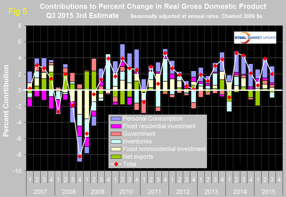
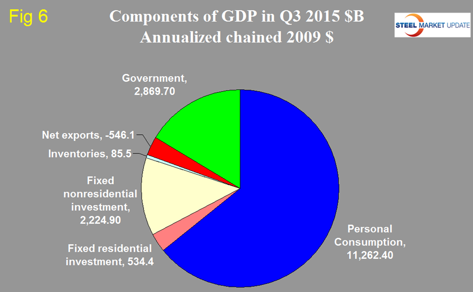
The last time that inventories made a major negative contribution was Q1 2014. Net exports were a major drag in Q4 2014 and Q1 2015 but the total effect in Q2 and Q3 2015 was almost a wash. The contribution of personal consumption at 2.04 percent was down from 2.42 percent in the 2nd quarter. Personal consumption includes goods and services, the goods portion of which includes both durable and non-durables. Government expenditures contributed 0.32 percent to growth in Q3 down from 0.46 percent in Q2. The contribution of fixed residential investment at 0.27 percent in Q3 has been fairly consistent for the last six quarters. The contribution of fixed nonresidential investment has been more variable and declined from 0.53 percent in Q2 to 0.33 percent in Q3. Inventories which had contributed positive 0.02 percent in Q2 contributed negative 0.71 percent in Q3. Over the long run inventory changes are a wash and simply move growth from one period to another. Figure 6 shows the breakdown of the $16 trillion economy.

On November 30th MAPI (Manufacturers Alliance for Productivity and Innovation) published the following on GDP and productivity which we at SMU have paraphrased:

In the U.S., potential GDP—the amount output can rise without increasing inflation—has slowed markedly since the 1980s and 1990s, when inflation-adjusted potential GDP was 3.3 percent a year. The potential growth rate embedded in today’s economic forecasts is much lower; for example, the Congressional Budget Office’s August 2015 federal budget update projected a 2.1 percent annual rate for the next 10 years. A recent Federal Reserve staff forecast says annual potential GDP growth is only 1.75 percent in the next five years. Potential GDP growth is composed of two basic building blocks—labor force growth and labor productivity growth.

Some pessimists, such as Robert Gordon of Northwestern University, believe that less innovation, reductions in labor quality improvement, and weak capital accumulation mean that potential growth could be as low as 1.4 percent annually through 2020.

A slow potential GDP growth rate has important ramifications for individuals and firms, particularly if the deceleration is due more to sluggish productivity growth than labor force demographics. If productivity is the cause, the reduced pace of growth in labor compensation and consumer spending over time impedes improvements to standards of living.

Low potential growth also reduces tax collection, increases our government debt burden, concentrates the burden of funding social welfare entitlements on workers, and causes firms to ratchet down capacity plans and thus invest less over time.

Most economists agree that the government statistics on output and productivity are not accurately measuring innovation such as internet products, software, and the sharing economy. But even on the miss-measurement point there are differences in opinion as to the degree of underestimation.

SMU Comment: On December 10th the BEA released quarterly GDP growth statistics by state through Q2 2015. We intend to perform a detailed analysis of this data and to report our findings next month. In the meantime we include here as Figure 7 the BEA geographical chart of state GDP.

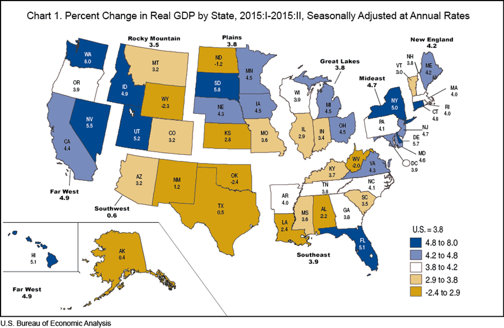
It seems to us at SMU that regional GDP combined with the regional job creation that we already report would provide a valuable matrix for the evaluation of local business conditions.