Gross Domestic Product Q4 2015 First Estimate

The annualized growth rate in the first estimate of the fourth quarter was 0.69 percent, down from 1.99 percent, in the 3rd quarter and down from 3.91 percent in Q2. Normally there are two revisions of the first estimate and sometimes three. Revisions to the first three quarters of 2015 were +0.4 percent, +1.59 percent and +0.5 percent respectively. GDP is measured and reported in chained 2009 dollars and in the first estimate of Q4 was $16.442 trillion. The growth calculation is misleading because it takes the Q over Q change and multiplies by 4 to get an annualized rate. This makes the high quarters higher and the low quarters lower. Figure 1 clearly shows this effect.

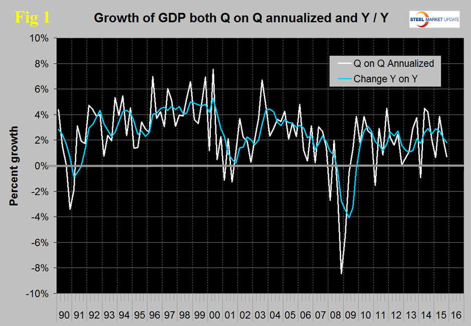
The blue line is the trailing 12 months growth and the white line is the headline quarterly result. On a trailing 12 month basis year over year, GDP was 1.8 percent higher in the fourth quarter of 2015 than it was in Q4 2014. In the last five years, since Q1 2011 the trailing 12 month growth of GDP has ranged from a high of 2.88 percent to a low of 1.07 percent therefore the latest result is on the low side of central within this variability.

We have commented in two of our recent reports (Housing starts and truck production) that we don’t think a recession is imminent. On January 29th Scott Grannis wrote: Because of the way the Fed conducts monetary policy, the Treasury yield curve can tell us a lot about the market’s expectations for economic growth and inflation. Since the Fed can only control short-term rates, observing longer-term rates can tell us a lot about the market’s expectations for the future of Fed policy. Figure 2 shows the history of two- and 10-year Treasury yields and the difference between the two, which is the slope of the yield curve. It also shows the last four recessions.

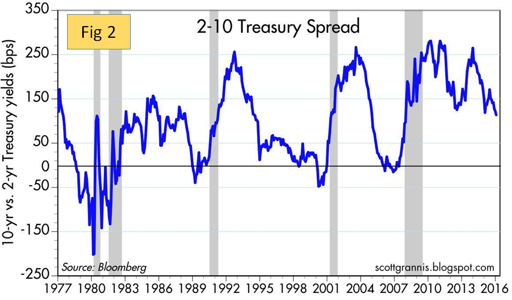
Note that the slope of the yield curve typically flattens or inverts (becomes negative) in advance of recessions. This is the bond market’s way of saying that emerging weakness in the economy is putting a lid on the Fed’s ability to raise short-term rates, and that it is increasingly likely that the Fed’s next move will be to cut, rather than raise, rates. The current slope of the yield curve is not unusual at all, and is typical of the middle part of a business expansion. The market doesn’t believe the economy is going to be weak enough to warrant lower short-term rates for the foreseeable future.

Figure 3 shows the headline quarterly results since 1990 and the latest IMF forecast through 2020.

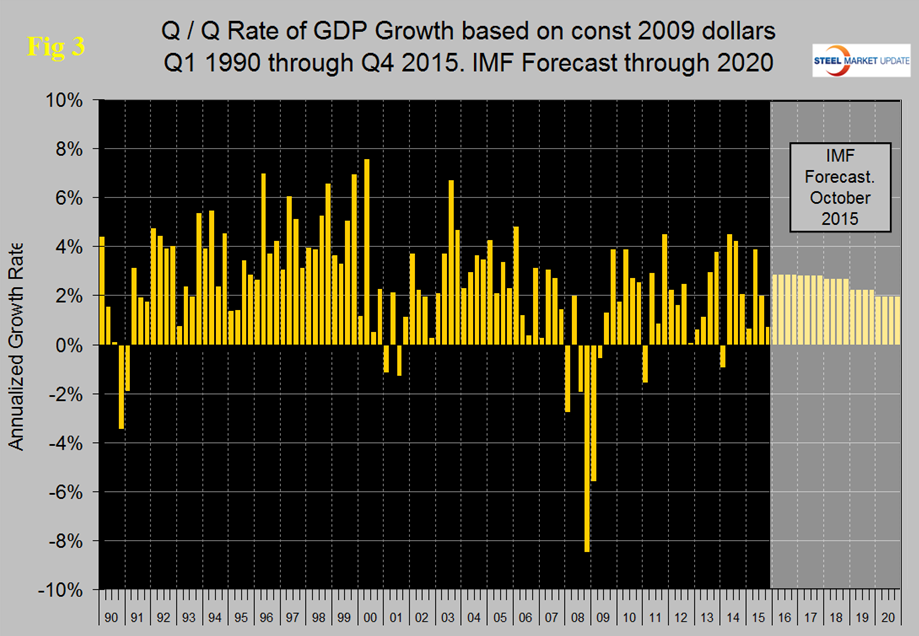
In their October revision, the IMF downgraded their forecast of US growth in 2015 from their April estimate of 3.14 percent to 2.57 percent and downgraded 2016 from 3.06 percent to 2.84 percent.

Historically it has been necessary to have about a 2.5 percent growth in GDP to get any growth in steel demand so this IMF forecast suggests a status quo through next year for our businesses.

There are six major subcomponents of the GDP calculation and the magnitude of these is shown in Figure 4.

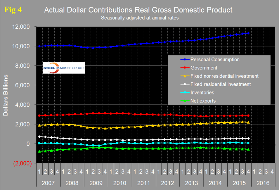
Personal consumption is dominant and in Q4 accounted for 68.86 percent of the total. Figure 5 shows the change in the major subcomponents of GDP in Q4 2015.

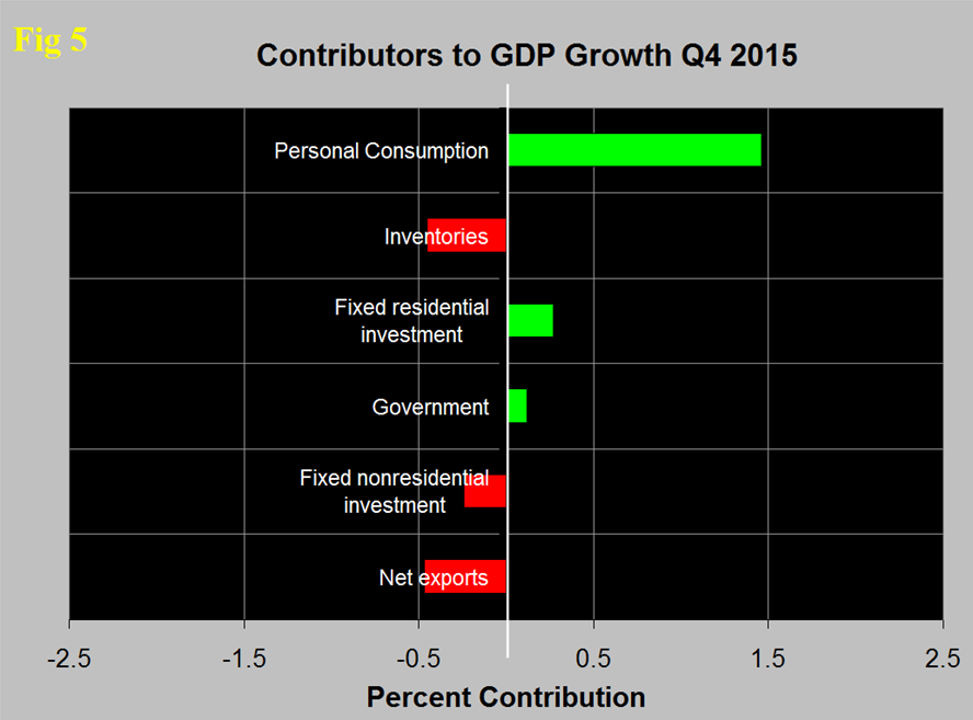
This shows how dominant the contribution of personal consumption was in the 4th quarter and also that the change in private inventories was a major detractor. Declining inventories have a negative effect on the overall GDP calculation. Net exports also reduced the overall result by 0.47 percent. The effect of net exports has been very erratic. In Q1 they contributed negative 1.92 percent and in Q2 positive 0.18 percent. Figure 6 shows the same data as Figure 5 extended back through Q1 2007 and describes the quarterly change in the six major subcomponents of GDP.

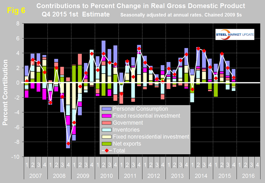
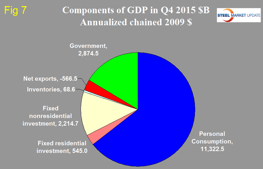
Prior to the latest two quarters of data, the last time that inventories made a major negative contribution was Q1 2014. Over the long run inventory changes are a wash and simply move growth from one period to another. The contribution of personal consumption at 1.46 percent was down from 2.04 percent in the 3rd quarter. Personal consumption includes goods and services, the goods portion of which includes both durable and non-durables. Government expenditures contributed 0.12 percent to growth in Q4 down from 0.32 percent in Q3. The contribution of fixed residential investment at 0.27 percent in Q4 was unchanged from Q3 and has been fairly consistent for the last seven quarters. The contribution of fixed nonresidential investment has been more variable and declined from positive 0.33 percent in Q3 to negative 0.24 percent in Q4. This is disturbing because it is supportive of the Dodge nonresidential starts data and is at odds with the recent Commerce Department construction put in place results. Inventories which had contributed negative 0.71 percent in Q3 contributed negative 0.45 percent in Q4. Figure 7 shows the breakdown of the $16 trillion economy.

SMU Comment: We have observed frequently in our SMU reports that steel demand has not been where it should be based on several previously indicative benchmark indicators and that a decline in inventories throughout the supply chain was likely a major contributing factor. This GDP data would seem to be supportive of that view as an inventory reduction has detracted from GDP for the last half of 2015.