

Market Data

September 30, 2016
Gross Domestic Product for Q2 2016 - Third Estimate
Written by Peter Wright
The annualized GDP growth rate in the third estimate of the second quarter of 2016 was 1.41 percent which was slightly above the consensus expectation of 1.3 percent and an improvement from the first estimate which was 1.2 percent. GDP is measured and reported in chained 2009 dollars and in the third estimate of Q2 was $16.583 trillion. The growth calculation is misleading because it takes the quarter over quarter change and multiplies by 4 to get an annualized rate. This makes the high quarters higher and the low quarters lower. Figure 1 clearly shows this effect.
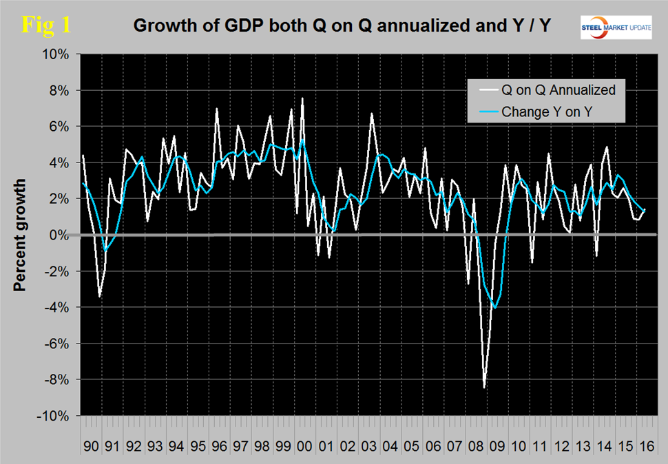
The blue line is the trailing 12 months growth and the white line is the headline quarterly result. Occasionally these measures coincide which was the case in the second quarter. On a trailing 12 month basis, GDP was 1.28 percent higher in Q2 2016 than it was in Q2 2015. In the last six years, since Q1 2011 the trailing 12 month growth of GDP has tracked between a high of 2.88 percent to a low of 1.07 percent therefore the latest result remains at the low side of this range.
Figure 2 shows the headline quarterly results since 1990 and the latest IMF forecast through 2020.
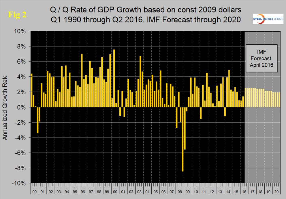
In their April revision, the IMF downgraded their forecast of US growth in 2016 from their October 2015 estimate of 2.84 percent to 2.4 percent and downgraded 2017 from 2.80 percent to 2.50 percent. Early next month (October) we will have access to the latest IMF projections and it looks as though a further reduction in expectations will occur.
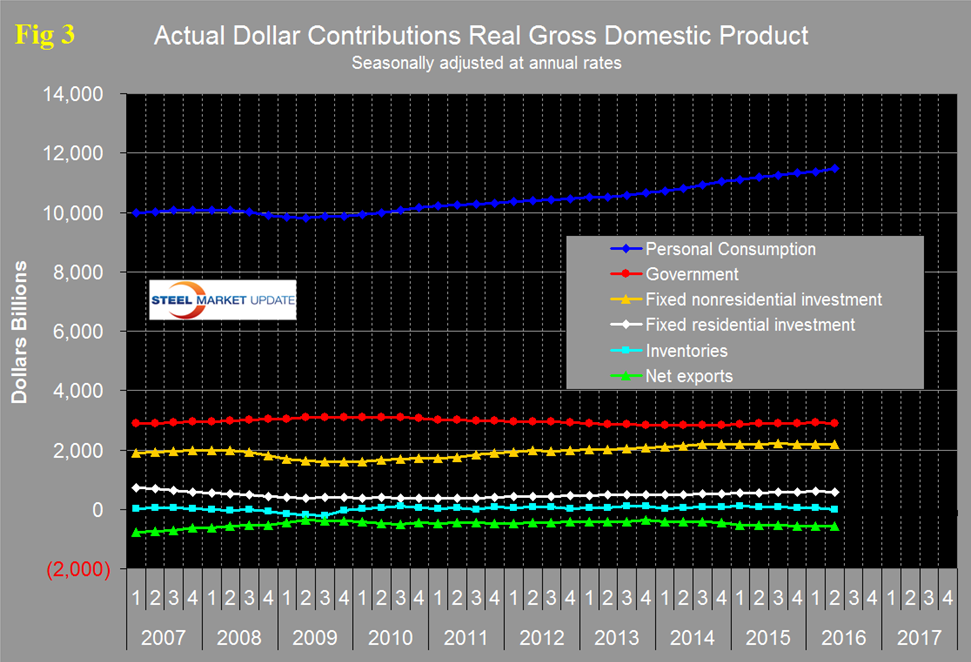
There are six major subcomponents of the GDP calculation and the magnitude of these is shown in Figure 3.
Personal consumption accounted for 69.3 percent of the total in the latest data and made its highest contribution to growth since Q4 2014. Retail sales again surprised on the upside in June, suggesting consumer spending growth may be gaining momentum.
Figure 4 shows the change in the major subcomponents of GDP in Q2 2016 and the dominance of personal consumption as a growth driver.
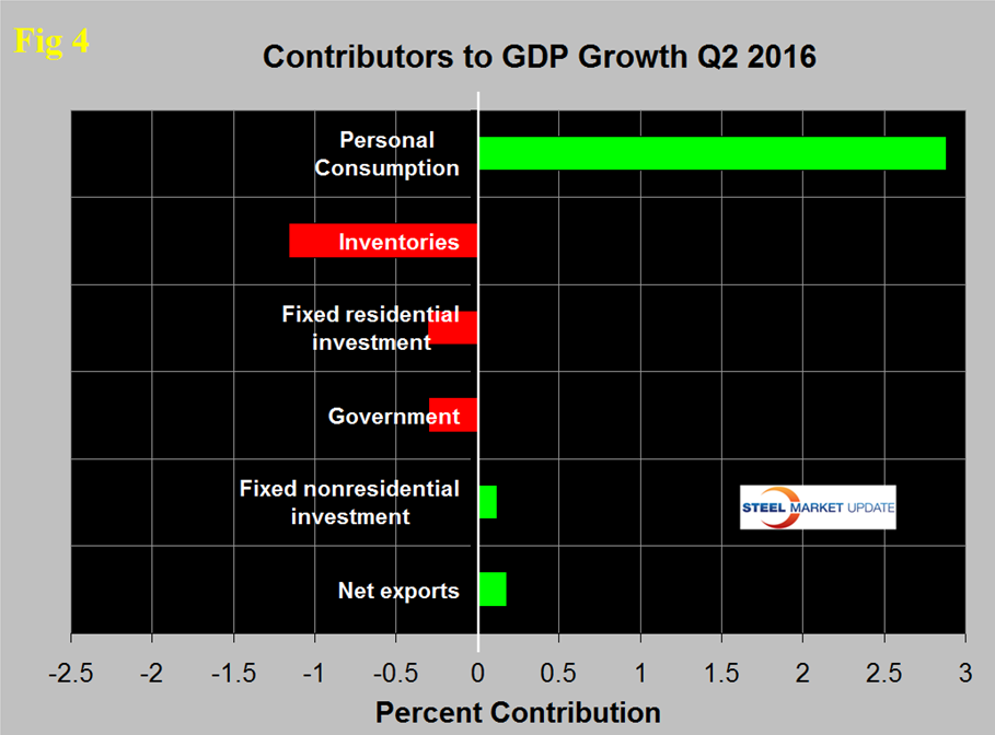
The change in inventories was the greatest detractor with a contribution of negative 1.16 percent. Declining inventories have a negative effect on the overall GDP calculation and this has been the case for the last five quarters. Over the long run inventory changes are a wash and simply move growth from one period to another. When a decline in one period is subtracted from growth, it can often be a healthy indicator for future periods. Such a decline suggests that there are lower levels of overall inventories which will set the stage for inventory increases – which will then add to GDP growth in the future. Residential construction made a negative contribution in Q2 as non-residential which includes infrastructure made a small positive contribution. Net exports made a positive contribution in Q2 and added 0.18 percent. Since US trade is net negative we don’t understand this result but we reproduce here what was reported. Figure 5 shows the contributors to GDP extended back through Q1 2007 and describes the quarterly change in the six major subcomponents.
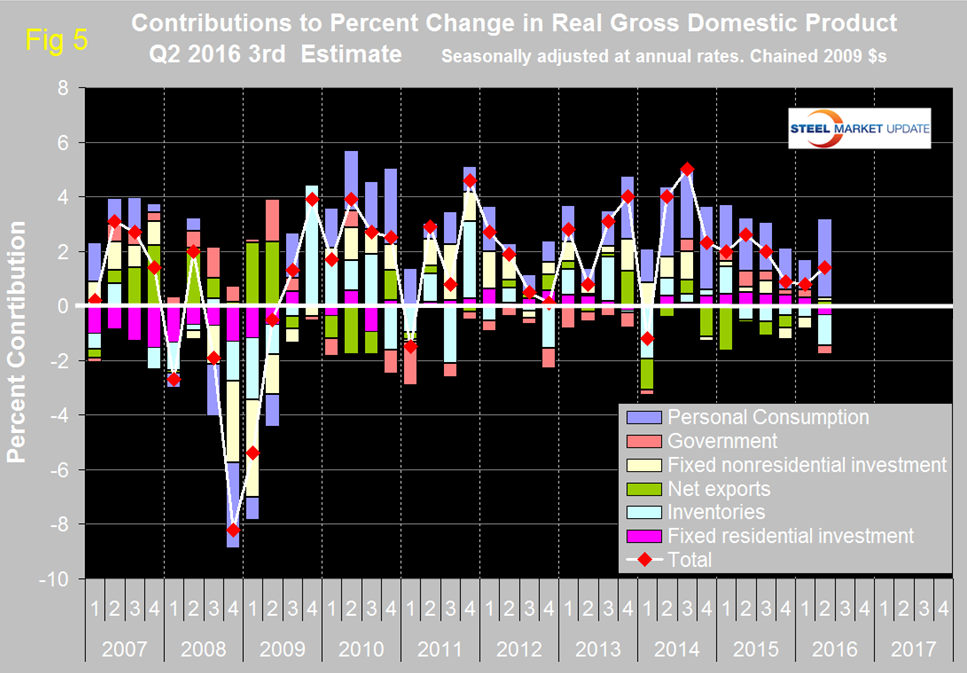
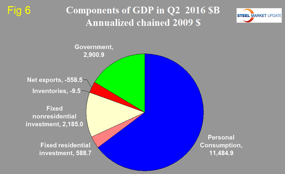
In this latest data the negative contribution of inventories was the greatest since Q1 2014. The contribution of personal consumption at 2.88 percent was up from 1.11 percent in the first quarter and the highest since Q4 2014. Personal consumption includes goods and services, the goods portion of which includes both durable and non-durables. Government expenditures contributed negative 0.3 percent in Q2 down from positive 0.28 percent in Q1. The contribution of fixed residential investment at negative 0.31 percent was the first time that this component detracted from GDP since Q1 2014. Figure 6 shows the breakdown of the $16.6 trillion economy.
SMU Comment: Historically it has been necessary to have about a 2.5 percent growth in GDP to get any growth in steel demand so this latest estimate of GDP doesn’t suggest any improvement in the steel market in the immediate future. This relationship is a long term average and in reality steel is much more volatile than GDP. If GDP takes a dive then steel demand craters and if GDP takes a sudden upturn steel soars. Neither of these extremes is evident at present.