Gross Domestic Product for Q2 2015, First Estimate

In the big picture, the change (delta) in GDP is equal to the change in population plus the change in productivity, that is Δ GDP = Δ Population + Δ Productivity. The BEA has been criticized for the way they do seasonal analysis which has tended to penalize the first quarter. Revisions were made retrospectively in this latest release with the result that Q1 2015 was revised up from negative 0.2 percent to positive 0.6 percent.

The annualized growth rate in the first estimate of the 2nd quarter was 2.3 percent, up from 0.6 percent in Q1. GDP is measured and reported in chained 2009 dollars and in Q2 was estimated to be $16.270 trillion. The calculation is slightly misleading because it takes the quarter over quarter growth and multiplies by 4 to get an annualized rate. This makes the high quarters higher and the low quarters lower. Figure 1 clearly shows this effect.

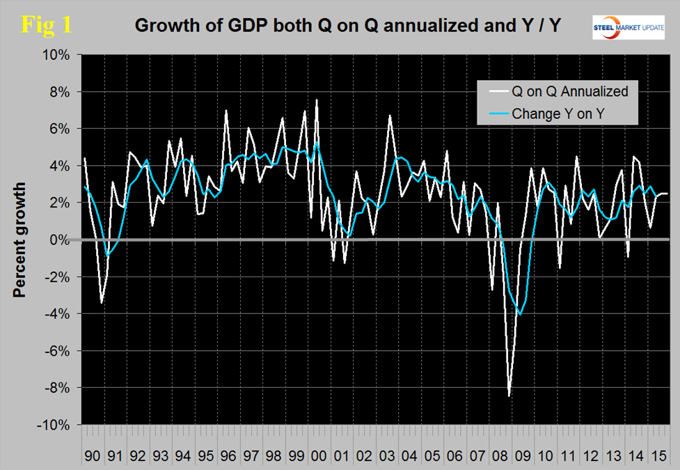
The blue line is the trailing 12 months growth and the white line is the headline quarterly result, this quarter these lines have coincided but that is not normally the case. On a year over year basis GDP was 2.32 percent higher in the 2nd quarter than it was in Q2 2014 and that result is in line with performance since Mid-2010.

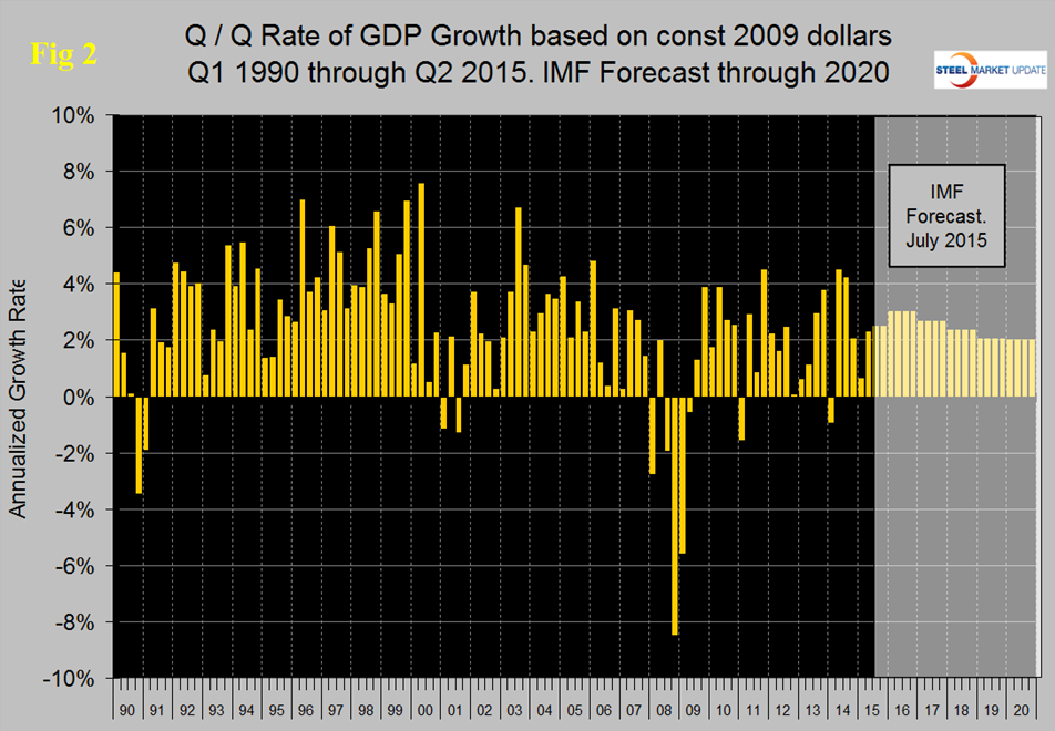
Figure 2 shows the headline quarterly results since 1990 and the latest IMF forecast through 2020.

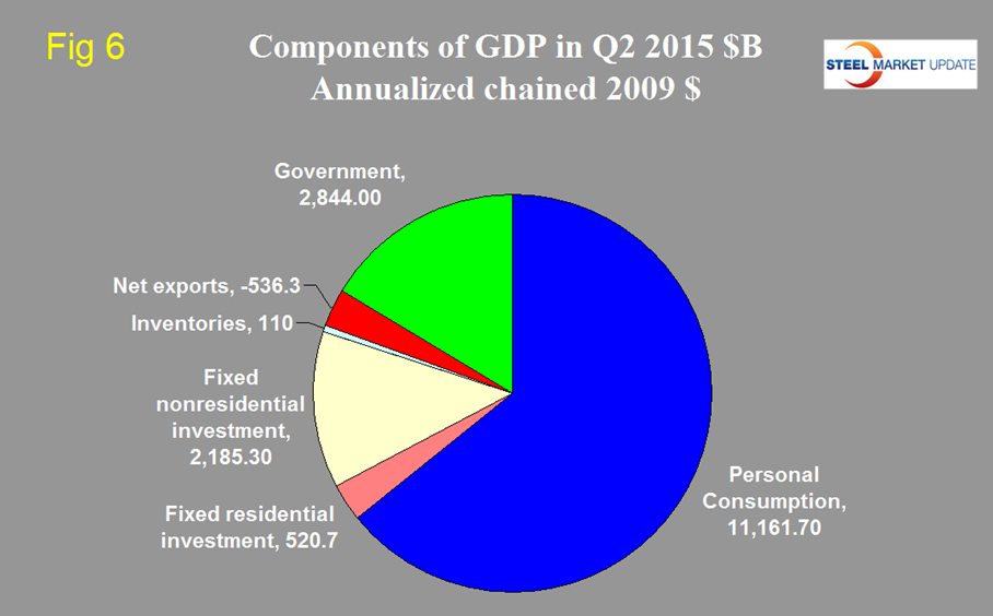
There are six major sub-components of the GDP calculation and the magnitude of these is shown in Figure 3.

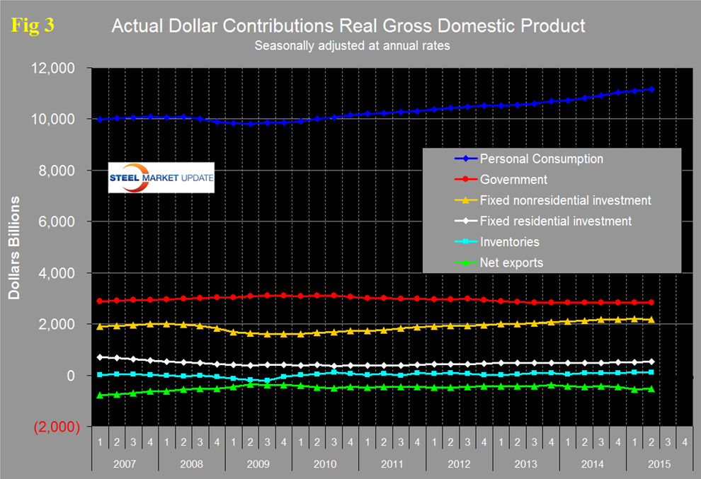
Personal consumption is dominant and in Q2 accounted for 68.60 percent of the total. Figure 4 shows the change in the major sub-components of GDP in Q2 2015.

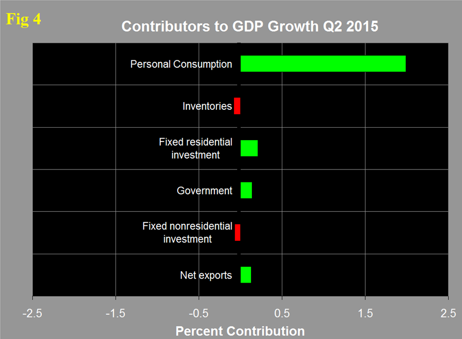
This shows how dominant the contribution of personal consumption was in the 2nd quarter with all other components close to a wash. Figure 5 shows the same data as Figure 4 extended back through Q1 2007 and describes the quarterly change in the six major sub-components of GDP.

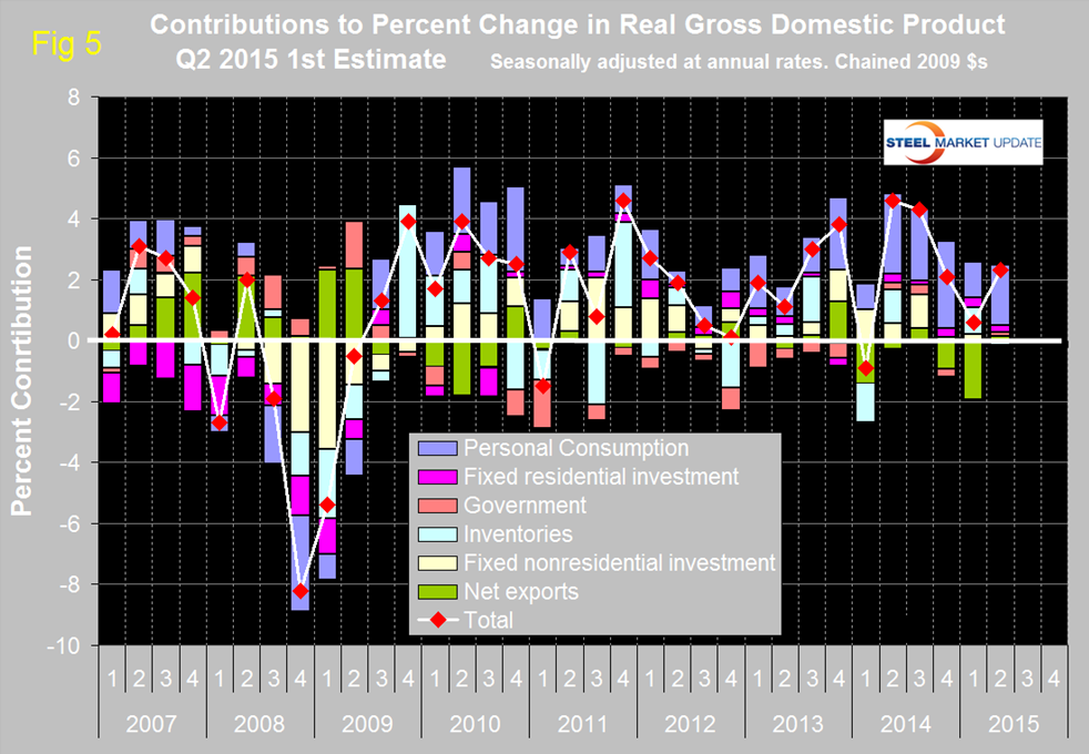
In the latest data there has been a dramatic change in net exports for which we have seen no explanation in our other investigations. In Q1 net exports contributed negative 1.92 percent and in Q2 contributed positive 0.13 percent. The contribution of personal consumption increased from 1.19 percent in Q1 to 1.99 in Q2. Personal consumption includes goods and services, the goods portion of which includes both durable and non-durables. Government expenditures contributed negative 0.1 percent to growth in Q1 and positive 0.14 percent in Q2. The contribution of fixed residential investment declined from 0.32 percent to 0.21 percent and the contribution of fixed nonresidential investment declined from 0.2 percent to negative 0.07 percent. Inventories which had contributed negative 0.87 in Q1 contributed negative 0.08 percent in Q2. Increasing inventories make a positive contribution to GDP and over the long run inventory changes are a wash and simply move growth from one period to another. Figure 6 shows the breakdown of the $16 trillion economy.

The official press release from the BEA reads as follows:

Real gross domestic product — the value of the production of goods and services in the United States, adjusted for price changes — increased at an annual rate of 2.3 percent in the second quarter of 2015, according to the “advance” estimate released by the Bureau of Economic Analysis. In the first quarter, real GDP increased 0.6 percent (revised). The Bureau emphasized that the second-quarter advance estimate released today is based on source data that are incomplete or subject to further revision by the source agency. The “second” estimate for the second quarter, based on more complete data, will be released on August 27, 2015.

The increase in real GDP in the second quarter reflected positive contributions from personal consumption expenditures (PCE), exports, state and local government spending, and residential fixed investment that were partly offset by negative contributions from federal government spending, private inventory investment, and nonresidential fixed investment. Imports, which are a subtraction in the calculation of GDP, increased.

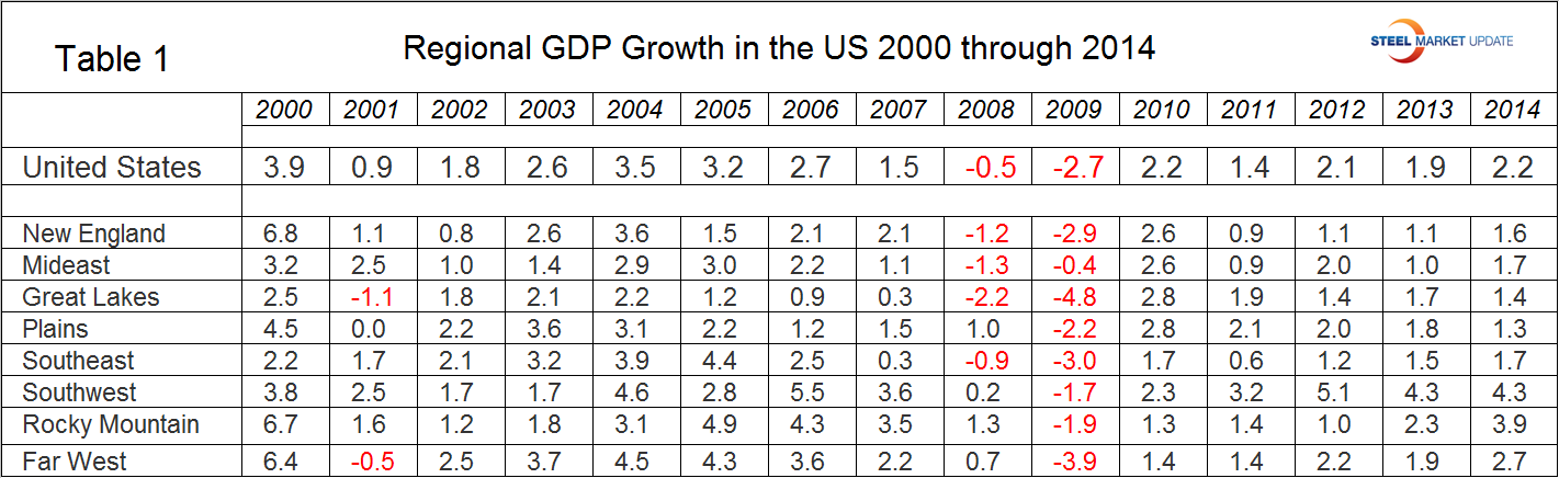
Regional GDP growth in the US. The Bureau of Economic Analysis is developing GDP data by region and state. On June 10th they published annual data through 2014. We don’t know at this point if they are going to break this data down into quarterly results but we will investigate this further. In the meantime here is a first look at GDP by region (Table 1).

SMU Comment: We have reported frequently in the past on the relationship between GDP and steel consumption. Steel growth follows economic growth but is very much more volatile. In addition over the long run about a 2.5 percent growth of GDP is necessary to get any growth in steel consumption. Based on the trailing 12 month growth of GDP which in Q2 was 2.32 percent we can expect steel consumption to be fairly stable in H2 2015. The IMF forecast for 2015 which in our last update was + 3.09 percent was revised down to 2.5 percent in July which if accurate suggests no change in steel demand.