Gross Domestic Product Q3 2015 First Estimate

The annualized growth rate in the first estimate of the third quarter was 1.49 percent, down from 3.91 percent, in the third estimate of Q2. GDP is measured and reported in chained 2009 dollars and in the first estimate of Q3 was $16.394 trillion. The growth calculation is misleading because it takes the Q over Q change and multiplies by 4 to get an annualized rate. This makes the high quarters higher and the low quarters lower. Figure 1 clearly shows this effect.

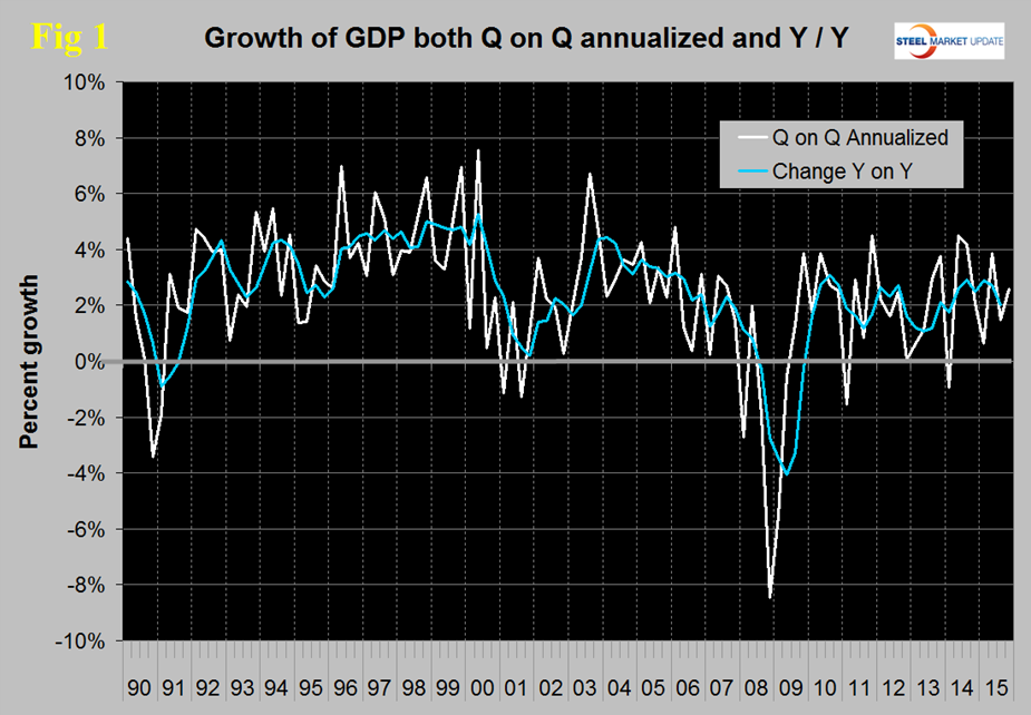
The blue line is the trailing 12 months growth and the white line is the headline quarterly result. On a trailing 12 month basis year over year, GDP was 2.03 percent higher in the third quarter than it was in Q3 2014. Since Q1 2011 the trailing 12 month growth of GDP has ranged from a high of 2.88 percent to a low of 1.07 percent therefore the latest result is central within this variability.

Figure 2 shows the headline quarterly results since 1990 and the latest IMF forecast through 2020.

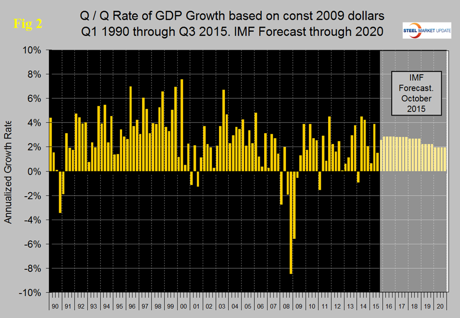
In their October revision, the IMF downgraded their forecast of US growth in 2015 from their April estimate of 3.14 percent to 2.57 percent and downgraded 2016 from 3.06 percent to 2.84 percent.

Historically it has been necessary to have about a 2.5 percent growth in GDP to get any growth in steel demand so this forecast suggests a status quo through next year for our businesses.

There are six major subcomponents of the GDP calculation and the magnitude of these is shown in Figure 3.

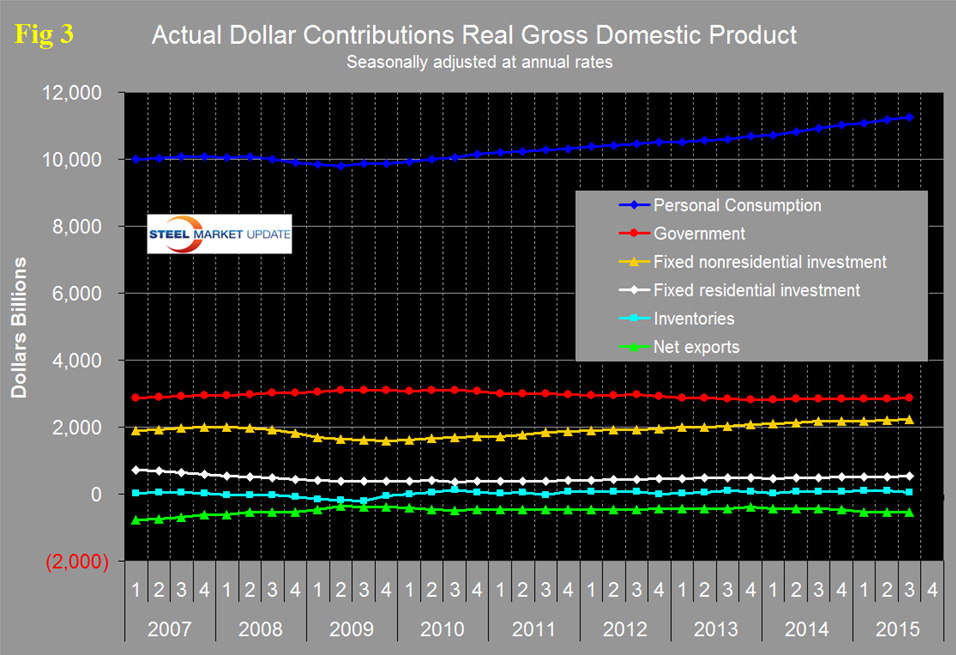
Personal consumption is dominant and in Q3 accounted for 68.74 percent of the total. Figure 4 shows the change in the major subcomponents of GDP in Q3 2015.

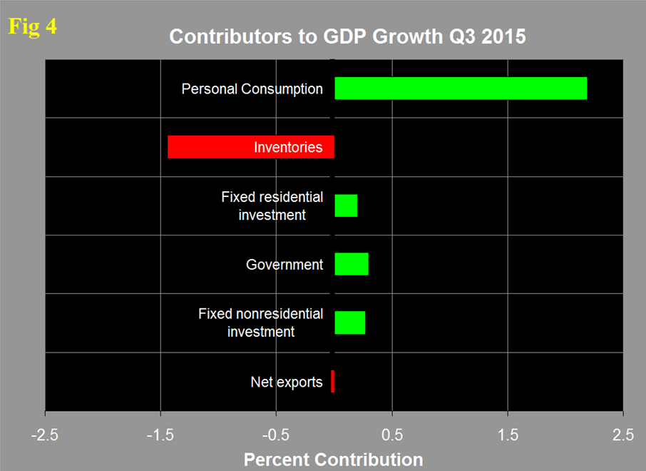
This shows how dominant the contribution of personal consumption was in the third quarter and also that the change in private inventories was a major detractor. Declining inventories have a negative effect on the overall GDP calculation. Figure 5 shows the same data as Figure 4 extended back through Q1 2007 and describes the quarterly change in the six major subcomponents of GDP.

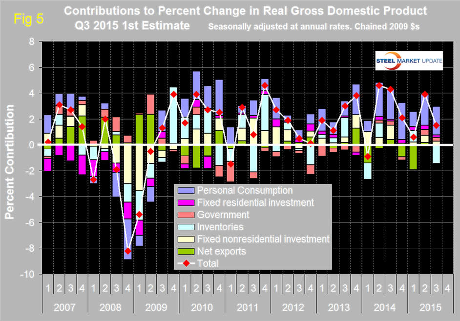
The last time that inventories made a major negative contribution was Q1 2014 and in the latest data the inventory component was the worst since Q4 2012. Net exports which made a negative contribution in Q4 2014 and Q1 2015 were almost a wash in Q3. The contribution of personal consumption at 2.19 percent was down from 2.42 percent in the second quarter. Personal consumption includes goods and services, the goods portion of which includes both durable and non-durables. Government expenditures contributed 0.3 percent to growth in Q3 down from 0.46 percent in Q2. The contribution of fixed residential investment at 0.30 percent in Q3 has been fairly consistent for the last six quarters. The contribution of fixed nonresidential investment has been more variable and declined from 0.53 percent in Q2 to 0.27 percent in Q3. Inventories which had contributed positive 0.02 percent in Q2 contributed negative 1.44 percent in Q3. Over the long run inventory changes are a wash and simply move growth from one period to another. Figure 6 shows the breakdown of the $16 trillion economy.

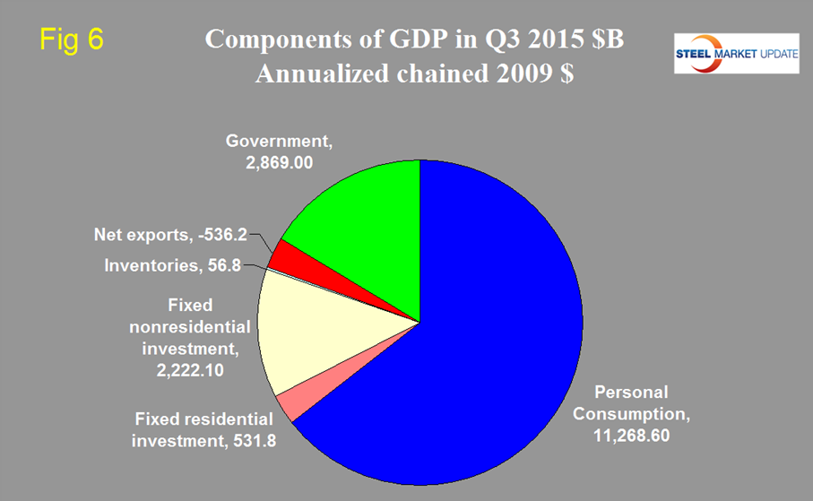
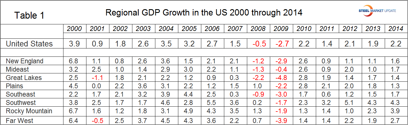
Table 1 shows the growth of regional GDP from 2000 through 2014. We have compiled this from the “prototype” date released by the BEA earlier this year.

On September second the BEA made the following statement and is improving the data to a quarterly level and by industry:

“The U.S. Bureau of Economic Analysis is releasing prototype quarterly gross domestic product (GDP) by state statistics for 2005–2014. The quarterly GDP by state statistics are released for 21 industry sectors and are in both current and inflation-adjusted chained (2009) dollars. The new data are intended to provide a fuller description of the accelerations, decelerations, and turning points in economic growth at the state level, including key information about the impact of industry composition differences across states. Relative to the August 2014 release, the new prototype statistics incorporate new and revised source data and cover an additional year of economic activity.

Statistics for the first quarter of 2015 are not being released as BEA continues to evaluate its methodology based on data users’ comments and evaluations received after the first release of prototype quarterly GDP by state statistics last September.

The following highlights for 2014 demonstrate how the new quarterly GDP by state statistics supplement the detail on state-level economic activity provided by annual GDP by state statistics.

In 2014:
– Real GDP increased in all eight BEA regions. However, in the first quarter of 2014 GDP declined in five of the eight regions. The Plains region declined the most primarily due to a decline in agriculture, forestry, fishing, and hunting.
– The Southwest region was the fastest growing region primarily due to strong growth in mining during the third quarter.
– North Dakota was the fastest growing state, but a slowdown in mining contributed to much slower real GDP growth rates in the last two quarters compared with the peak growth rate in the second quarter.
– Mississippi and Alaska declined. However, both of these states ended 2014 with growth in the fourth quarter. Growth in Mississippi was primarily due to strong growth in non-durable goods manufacturing and Alaska primarily due to growth in mining.

Most states experienced quarters of both positive and negative real GDP growth. However, in a few states, such as Utah and Washington, real GDP consistently grew over all four quarters.”

SMU Comment: We are hopeful that the BEA will continue regular data for state level GDP. Table 1 shows how regional recessions usually are, with the exception of the “Great” one. It seems to us at SMU that regional GDP combined with the regional job creation that we already report would provide a valuable matrix for the evaluation of local business conditions.